Stereo vision and disparity maps (in Julia)

I’ve been working a lot recently with stereo vision and wanted to go through the basics of how disparity is calculated. I’m partially doing this as an excuse to get better at Julia (v1.9.3 used here).

You can view the notebook for this blog post on Github:

Introduction

In much the same way that we as humans can have depth perception by sensing the difference in the images we see between our left and right eyes, we can calculate depth from a pair of images taken from different locations, called a stereo pair.

If we know the positions of out cameras, then we can use matching points in our two images to estimate how far away from the camera those points are.

Taking a look at the image below (from OpenCV):

https://docs.opencv.org/4.x/dd/d53/tutorial_py_depthmap.html

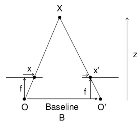
If we have two identical cameras, at points \(O\) and \(O'\) at a distance \(B\) from each other, with focal length \(f\), we can calculate the distance (\(Z\)) to object \(X\) by using the disparity between where the object \(X\) appears in the left image (\(x\)) and where it appears in the right image (\(x'\)).

In this simple case, the relation between disparity and distance is simply:

\[\begin{equation} disparity = x - x' = \frac{Bf}{Z} \end{equation}\]

If we know \(B\) an \(f\), then we can rearrange this to give us distance as a function of disparity:

\[\begin{equation} Z = \frac{Bf}{x - x'} \end{equation}\]

You might notice that in case the disparity is zero, you will have an undefined result. This is just due to the fact that in this case the cameras are pointing in parallel, so in principle a disparity of zero should not be possible.

The general case is more complicated, but we will focus on this simple setup for now.

We can define the function as:

function distance_from_disparity(B, f, disparity)
    B*f/disparity
end

distance_from_disparity (generic function with 1 method)

Where \(B\) and \(disparity\) are measured in pixels, and \(f\) is measured in centimeters.

There is an inverse relation between distance and disparity:

using Plots

disparities = range(1, 50, length=50)
distances = distance_from_disparity.(2000, 0.1, disparities)

plot(disparities, distances, label="Distance [cm]")
xlabel!("Disparity")
ylabel!("Distance [cm]")

So once we have a disparity, it’s relatively straightforward to get a distance. But how do we find disparities?

Disparity maps

We usually represent the disparities for a given pair of images as a disparity map, which is an array with the same dimensions as (one of) your images, but with disparity values for each pixel.

In principle, this is a two-dimensional problem, as an object might be matched to a point that has both a horizontal and vertical shift, but luckily, you can always find a transformation to turn this into a one dimensional problem.

The cartoon below illustrates what a disparity map might look like: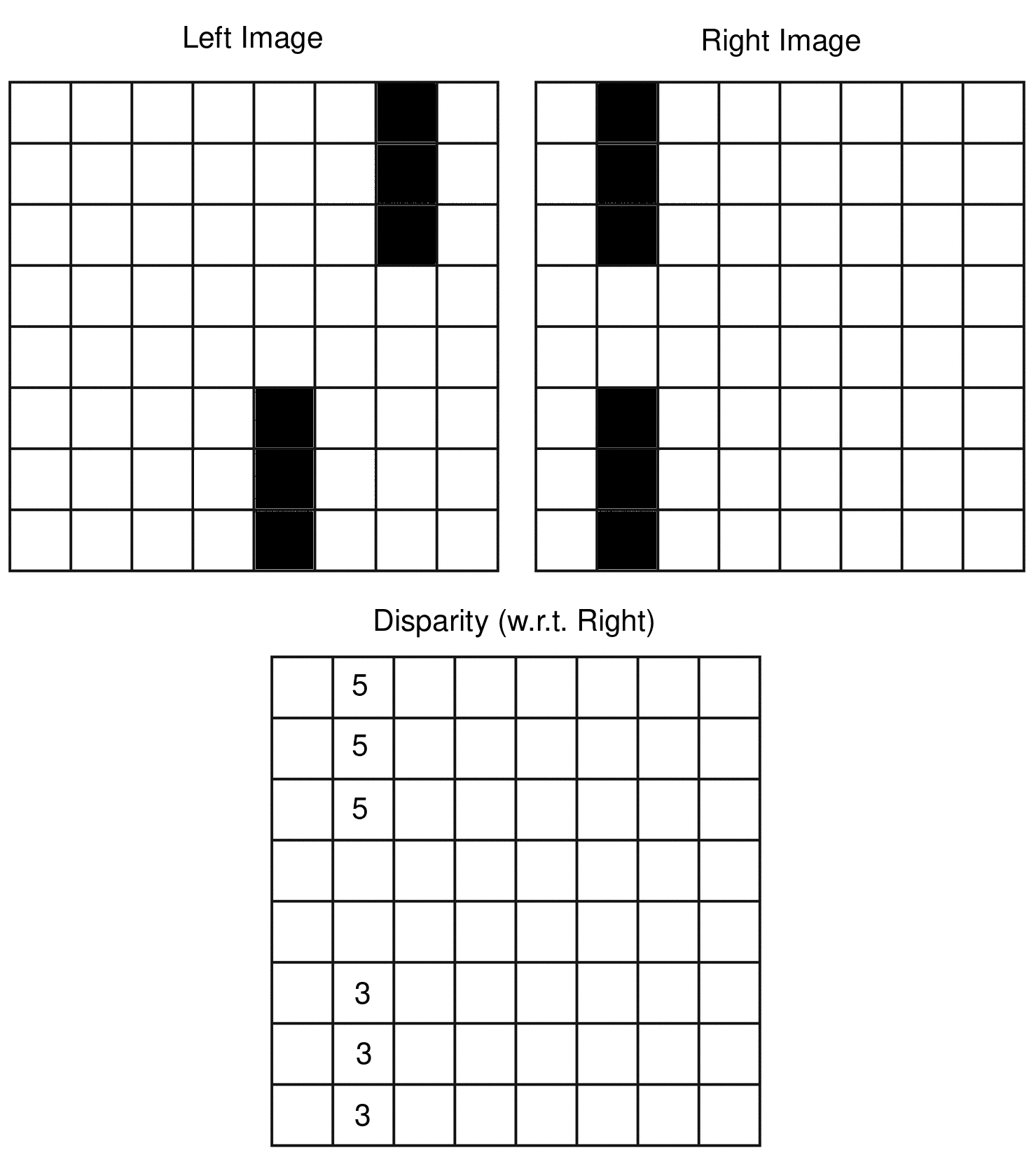

Above, we calculate the disparity with respect to the right image (you can do it with respect to the left image as well), and as you can see the disparity map tells us how many pixels to the right each object shifted in the left image vs the right image.

For a set of images (taken from the Middlebury Stereo Datasets):

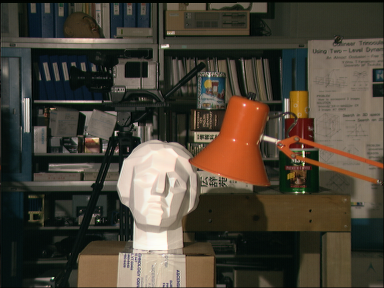
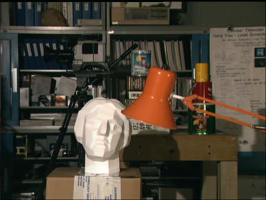
The corresponding disparity map can be visualized as follows:

https://vision.middlebury.edu/stereo/eval/newEval/tsukuba/

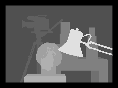
With darker pixels having lower disparity values, and brighter pixels having higher disparity values, meaning the dark objects are far away from the cameras, while the bright ones are close.

The ground truth disparity as shown above is usually calculated from LiDAR or some other accurate method, and our goal is to get as close as possible to those values using only the images above.

A naive approach

So let’s try and calculate disparity for the images above.
There are many, many approaches to calculating disparity, but let us begin with the most simple approach we can think of.
As a start, let us go through each pixel in the right image, and for that pixel, try and find the most similar pixel in the left image.

So let us try and take the squared difference between pixels values as our similarity metric. As we are going to be doing the same thing for every row of pixels, we are just going to define a function that does the basic logic, and then apply the same function to every case.

function smallest_diff(pixel, row, metric)

    disparity_candidates = metric.(pixel, row)
    # Minus one as Julia counts from 1
    argmin(disparity_candidates) - 1
end

smallest_diff (generic function with 1 method)

Let’s define a distance metric as the squared distance:

squared_difference = (x, y) -> sum((x-y).^2)

#9 (generic function with 1 method)

And as a test case let’s create the cartoon image we had above:

left_image = ones(Float64, (8, 8))
right_image = ones(Float64, (8, 8))
disparity = ones(UInt8, (8, 8))

right_image[2, 1] = 0
right_image[2, 2] = 0
right_image[2, 3] = 0
right_image[2, 6] = 0
right_image[2, 7] = 0
right_image[2, 8] = 0

left_image[7, 1] = 0
left_image[7, 2] = 0
left_image[7, 3] = 0
left_image[5, 6] = 0
left_image[5, 7] = 0
left_image[5, 8] = 0

Gray.(left_image')

Gray.(right_image')

Now we can try and match pixels in the right image to pixels in the left image.

# NOTE: Julia is column major, not row major like Python or C/C++, 
# so this looping is not optimal. But I'm going for clarity, not speed. 
for i in range(1, size(right_image)[1])
    for j in range(1, size(right_image)[2])
        disparity[j, i] = max(smallest_diff(right_image[j, i], left_image[j:end, i], squared_difference), 1)
    end
end
    

So how did we do?

Gray.(disparity'/5)

So the toy example works! The top line, which moved more pixels, shows up brighter (i.e. larger disparity values), and the lower line is dimmer.

So let’s move on to real images. We’ll start with the example case above, but for simplicity we’ll stick to grayscale at first:

using Images, FileIO

tsukuba_left_gray = Gray.(load("im3.png"))
tsukuba_right_gray = Gray.(load("im4.png"))


tsukuba_right_gray

"""
Iterrate over the rows of the right image. 
For each row, find the most similar pixel in the left image and return the difference in location for them (disparity). 
The similarity is defined by the provided metric. 
"""
function pixel_match(left_image, right_image, metric, max_disp)

    num_rows = size(right_image)[2]
    num_cols = size(right_image)[3]

    disparity = zeros((num_rows, num_cols))
    for i in range(1, num_rows)
        for j in range(1, num_cols)
            terminator = min(j+max_disp, num_cols)
            pixel = right_image[:, i, j]
            row = left_image[:, i, j:terminator]
            
            disparity[i, j] = max(smallest_diff(pixel, row, metric), 1)
        end
    end

    disparity
end

pixel_match

Redefining smallest_diff slightly…

function smallest_diff(pixel, row, metric)
    disparity_candidates = metric.(pixel, row)
    # Minus one as Julia counts from 1
    argmin(disparity_candidates)[2] - 1
end

smallest_diff (generic function with 1 method)

# Transform images to Float64 to avoid integer overflow when calculating metric. 
# Reshape to 3 dim array with 1 channel. Julia is channel first
array_size = (1, size(tsukuba_left_gray)...,)
tsukuba_left_gray_float = reshape(Float64.(tsukuba_left_gray), array_size)
tsukuba_right_gray_float = reshape(Float64.(tsukuba_right_gray), array_size)


tsukuba_disparity_gray = pixel_match(tsukuba_left_gray_float, tsukuba_right_gray_float,  squared_difference, 20);

So let’s see how we did?

max_plot_disp = 15
Gray.(tsukuba_disparity_gray / max_plot_disp)

Looking at the predicted disparity, we can see there is some vague resemblance to the input image, but we’re still pretty far from the target:

https://vision.middlebury.edu/stereo/eval/newEval/tsukuba/

A significant problem seems to be erroneous matches, especially in the background.

As you can imagine, we are only comparing single channel pixels values, and it’s very likely that we might just find a better match by chance. In grayscale we are only matching pixel intensity, and we have no idea whether something is bright green, or bright red.

So let’s try and improve the odds of a good match by adding colour.

tsukuba_left_rgb = load("im3.png")
tsukuba_right_rgb = load("im4.png")
 

tsukuba_left_rgb

tsukuba_left_rgb_float = Float64.(channelview(tsukuba_left_rgb))
tsukuba_right_rgb_float = Float64.(channelview(tsukuba_right_rgb))
tsukuba_disparity_rgb = pixel_match(tsukuba_left_rgb_float, tsukuba_right_rgb_float,  squared_difference, 20);

Gray.(tsukuba_disparity_rgb / max_plot_disp)

So, a slight improvement! There seem to be fewer random matches in the background, but still not that close to the desired outcome.

Is there more we can do?

Block matching

The obvious downside of the naive approach above is that it only ever looks at one pixel (in each image) at a time.
That’s not a lot of information, and also not how we intuitively match objects.

Look at the image below. Can you guess the best match for the pixel in the row of pixels below it?

Own work

Given only this information, it’s impossible for us to guess whether the green pixel matches with the pixels at location 3, 5 or 7.

If however I was to give you more context, i.e. a block of say 3x3 pixels, would this make things simpler?

Own work

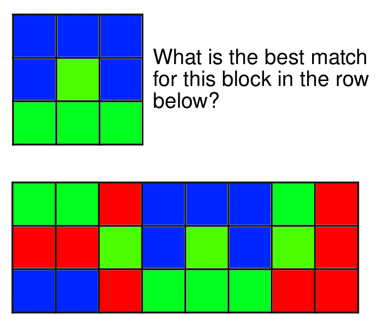
In this case, there is an unambiguous answer, which is the principle behind block-matching.

To confirm our idea that more context results in better matches, we can take a quick look at a row of pixels:

max_disp = 100
block_size = 0
i = 100
j = 220
test_row = tsukuba_left_rgb[i-block_size:i+block_size, j-block_size:j+max_disp];
test_block = tsukuba_right_rgb[i-block_size:i+block_size, j-block_size:j+block_size];
test_block

Given the pixel above, where in the row below do you think this pixel matches?
You would guess somewhere in the orange part on the left right? But which pixel exactly is almost impossible to say.

test_row

If we now take a block with more context:

block_size = 5
test_row = tsukuba_left_rgb[i-block_size:i+block_size, j-block_size:j+max_disp];
test_block = tsukuba_right_rgb[i-block_size:i+block_size, j-block_size:j+block_size];
test_block

And compare it to the row below, the location of the match becomes more obvious:

test_row

Calculating the difference metric for each point with different block sizes, we can clearly see that for low block sizes, the lowest metric value is ambiguous, while for larger block sizes it becomes more clear where exactly the best match is:

sum_squared_difference_rgb_block = (x, y) -> sum((x - y).^2)

function smallest_block_diff(block, row, metric, block_size)

    view_length = size(row)[3]
    disparity_candidates = zeros(view_length - 2*block_size)

    for i in range(block_size + 1, view_length - block_size )
        
        disparity_candidates[i-block_size] = metric(block, row[:, :, i-block_size:i+block_size])
    end
    disparity_candidates 

end

p1 = plot()
for b in [0, 2, 4]
    block_size = b
    i = 100
    j = 220
    max_disp = 100
    test_row = tsukuba_left_rgb[i-block_size:i+block_size, j-block_size:j+max_disp];
    test_block = tsukuba_right_rgb[i-block_size:i+block_size, j-block_size:j+block_size];
    x = Float64.(channelview(test_block))
    y = Float64.(channelview(test_row))
    diffs = smallest_block_diff(x, y, sum_squared_difference_rgb_block, block_size)

    norm_diffs = (diffs .- minimum(diffs))./maximum(diffs)

    plot!(p1, norm_diffs, label="Blocksize $block_size", linewidth=2)

end

p1

And now we are ready to define our block matching algorithm, much in the way we did our pixel matching algorithm:

function block_match(left_image, right_image, block_size, metric, max_disp)

    
    num_rows = size(left_image)[2]
    num_cols = size(left_image)[3]

    disparity = zeros((num_rows, num_cols))
    for i in range(block_size + 1, num_rows - block_size)
        for j in range(block_size + 1, num_cols - block_size)
            terminator = min(j+max_disp, num_cols)

            row_block_index = i-block_size:i+block_size
            col_block_index = j-block_size:j+block_size
            
            block = right_image[:, row_block_index, col_block_index]
            row = left_image[:, row_block_index, j-block_size:terminator]

            disparity_candidates = smallest_block_diff(block, row, metric, block_size)

            disparity[i, j] = max(argmin(disparity_candidates) -1, 1)
        end
    end

    disparity
end

block_match (generic function with 1 method)

Let’s see how this does on the full image in comparison to the pixel matching:

tsukuba_disparity_rgb = block_match(tsukuba_left_rgb_float, tsukuba_right_rgb_float, 2,  sum_squared_difference_rgb_block, 20);
Gray.(tsukuba_disparity_rgb / max_plot_disp)

Now we are getting somewhere! Compared to the earlier results we can now start making out the depth of the separate objects like the lamp, bust and camera.

There are still a few things we could do to improve our simple algorithm (like only accepting matches that have below a certain score for the metric), but I will leave those as an exercise to the reader.

Conclusions

Above we went through a basic introduction to stereo vision and disparity, and built a bare-bones block matching algorithm from scratch.

The above is pretty far away from the state of the art, and there are many more advanced methods for calculating disparity, ranging from relatively simple methods like block matching to Deep Learning methods.

Further reading

Below are some posts/guides I found informative:

• Introduction to Epipolar Geometry and Stereo Vision
  
• Stereo Vision: Depth Estimation between object and camera
  
• Depth Map from Stereo Images